|
This is going to be a two-part blog post. Here, we will simulate data for a capture-mark-recapture study, and then next time, we will analyze that data in JAGS. Here is the scenario: We are disease ecologists, and we want to understand the disease dynamics of our system. When we capture an individual, we assign it to a certain ‘state.’ A state in our case is a disease status, but can also be defined as a geographic location, an age, a breeding status, etc. Before we begin, I’d like to lay out some information: Our parameters of interest: state-specific apparent survival probability, recruitment probability, transition rates (i.e., movement between two ‘states’), abundance for each state, and population growth rate (depicted in Figure 1). 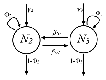 Figure 1. Graphical representation of our model describing the processes contributing to changes in abundance. Parameter names are explained in Table 1. The type of data we ‘collect’: capture-mark-recapture- where each individual is captured, uniquely marked (e.g., elastomer tags, pit tag, toe clips, etc.), and released. Then, each season, new individuals are marked, and old individuals are recaptured. When an individual is captured, we record its state. Our modeling approach: Multi-state Jolly-Seber Model Statistical framework: Bayesian For more information on these models, I highly recommend the book: Bayesian population analysis using WinBUGs by Marc Kéry and Michael Schaub. Table 1 Parameter definitions and symbols. 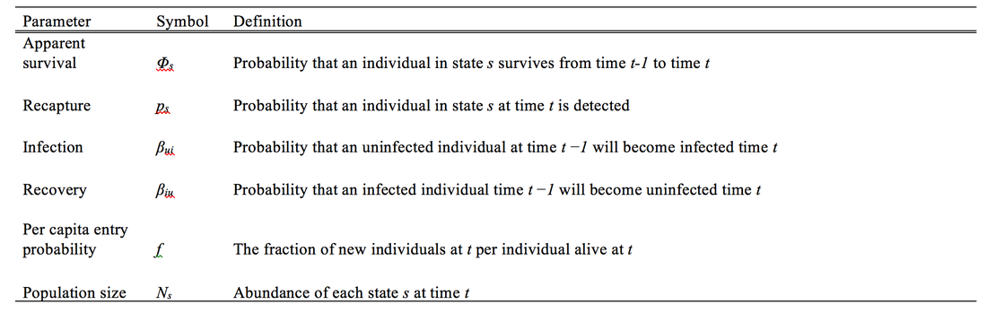 #--------------- R code starts here
#--- Survey conditions n.occasions <- 4 # Number of seasons #---- Population parameters # Super population size of uninfecteds N_U <- 250 # Super population size of infecteds N_I <- 200 # Super population size of all N <- N_U + N_I # Number of states n.states <- 4 # Number of observable states n.obs <- 3 #--- Define parameter values # Uninfected survival probability phi_U <- 0.9 # Infected survival probability phi_I <- 0.7 #------ Entry probability # Entry probability of uninfected hosts gamma_U <- (1/(n.occasions-1))/2 # Entry probability of infected hosts gamma_I <- (1/(n.occasions-1))/2 #------ Transition probability #(Uninfected to Infected) beta_UI <- 0.2 #(Infected to Uninfected) beta_IU <- 0.3 #------ Detection probability # Uninfected detection probability p_U <- 0.9 # Infected detection probability p_I <- 0.7 #---- 1. State process matrix #---- 4 state system # 1. Not entered # 2. Uninfected # 3. Infected # 4. Dead PSI.state <- array(NA, dim = c(n.states, n.states, N, n.occasions-1)) for(i in 1:N){ for(j in 1:n.occasions-1){ PSI.state[,,i,j] <- matrix(c(1 - gamma_U - gamma_I, gamma_U, gamma_I, 0, 0, phi_U * (1- beta_UI), phi_U * beta_UI, 1-phi_U, 0, phi_I * beta_IU, phi_I * (1- beta_IU), 1-phi_I, 0, 0, 0, 1), nrow = 4, ncol = 4, byrow = T) } } # 2. Observational process matrix #----- 3 observed states # 1. Seen uninfected # 2. Seen infected # 3. Not seen PSI.obs <- array(NA, dim = c(n.states, n.obs, N, n.occasions-1)) for(i in 1:N){ for(j in 1:n.occasions-1){ PSI.obs[,,i,j] <- matrix(c( 0, 0, 1, p_U, 0, 1- p_U, 0, p_I, 1- p_I, 0, 0, 1), nrow = 4, ncol = 3, byrow = T) } } #---- Function to simulate capture-recapture data simul.js <- function(PSI.state, PSI.obs, gamma_U, gamma_I, N, N_U, N_I){ n.occasions <- dim(PSI.state)[4] + 1 B_U <- rmultinom(1, N_U, rep(gamma_U, times = n.occasions)) B_I <- rmultinom(1, N_I, rep(gamma_I, times = n.occasions)) # Generate no. of entering hosts per occasion # N is superpopulation size B <- B_U + B_I CH.sur <- CH.p <- matrix(0, ncol = n.occasions, nrow = N) # Define a vector with the occasion of entering the population ent.occ_U <- ent.occ_I <- numeric() for (t in 1:n.occasions){ ent.occ_U <- c(ent.occ_U, rep(t, B_U[t])) ent.occ_I <- c(ent.occ_I, rep(t, B_I[t])) } ent.occ <- c(ent.occ_U, ent.occ_I) # Simulating survival for (i in 1:length(ent.occ_U)){ # For each individual in the superpopulation CH.sur[i, ent.occ_U[i]] <- 2 } for(i in (length(ent.occ_U)+1):length(ent.occ)){ CH.sur[i, ent.occ[i]] <- 3 } for (i in 1:N){ # Probability of capturing the individual during the first occasion if(CH.sur[i, ent.occ[i]] == 2){ CH.p[i, ent.occ[i]] <- 1 * rbinom(1, 1, p_U) }else{ CH.p[i, ent.occ[i]] <- 2 * rbinom(1, 1, p_I) } if (ent.occ[i] == n.occasions) next # If the entry occasion = the last occasion, go next for(t in (ent.occ[i]+1):n.occasions){ # for each occasion from entering 2 last occasion # Determine individual state history sur <- which(rmultinom(1, 1, PSI.state[CH.sur[i, t-1], , i, t-1]) == 1) CH.sur[i, t] <- sur # Determine if the individual is captured event <- which(rmultinom(1, 1, PSI.obs[CH.sur[i, t], , i, t-1]) == 1) CH.p[i, t] <- event } #t } #i #---- Reorder CH.p <- CH.p[ c(which(ent.occ == 1), which(ent.occ == 2), which(ent.occ == 3), which(ent.occ == 4)),] CH.sur <- CH.sur[ c(which(ent.occ == 1), which(ent.occ == 2), which(ent.occ == 3), which(ent.occ == 4)),] # Remove individuals never captured CH <- CH.p * CH.sur cap.sum <- rowSums(CH) never <- which(cap.sum == 0) if(length(never) > 0) { CH.p <- CH.p[-never,] } Nt <- numeric(n.occasions) # Calculate super population size by the simulated data for(i in 1:n.occasions){ Nt[i] <- length(which(CH.sur[,i] > 0)) } #----- CH <- CH.p CH[is.na(CH) == TRUE] <- 0 CH[CH == dim(PSI.state)[1]] <- 0 id <- numeric(0) for(i in 1:dim(CH)[1]){ # For each individual row z <- min(which(CH[i, ] != 0)) # which column is the lowest that does not = 0? ifelse(z == dim(CH)[2], id <- c(id, i), id <- c(id)) # keep a list of individuals only captured on last occasion } CH.sur[CH.sur == 0] <- 1 return(list(CH.p = CH.p[-id, ], CH.sur = CH.sur[-id,], B = B, Nt = Nt)) } # Execute simulation function sim <- simul.js(PSI.state = PSI.state, PSI.obs = PSI.obs, gamma_U = gamma_U, gamma_I = gamma_I, N = N, N_U = N_U, N_I = N_I) #----------------------------# Hope this was helpful and feel free to shoot me an email with any questions at [email protected]
24 Comments
|
Graziella DiRenzoBayesian Analyst sharing my experiences and code Archives
August 2018
Categories |
 RSS Feed
